Technical Report
Technical Report
This document elaborately demonstrates the process of data analysis and learning carried out in order to train an optimal model.
Read the data
The total number of data points in the dataset are 961. But there are missing values in the dataset and the rows corresponding to the missing values are removed. Thus the cleaned data has 830 rows.
import pandas as pd
import numpy as np

data = pd.read_csv('data.csv')
print('Number of rows before removing missing values: %d' % data.shape[0])
# Remove rows containing missing values.
cleanData = data.replace('?', np.nan).dropna().reset_index(drop=True)
cleanData = cleanData.astype('float64')


cleanData.describe()
Number of rows before removing missing values: 961
| BIRADS | Age | Shape | Margin | Density | Severity | |
|---|---|---|---|---|---|---|
| count | 830.000000 | 830.000000 | 830.000000 | 830.000000 | 830.000000 | 830.000000 |
| mean | 4.393976 | 55.781928 | 2.781928 | 2.813253 | 2.915663 | 0.485542 |
| std | 1.888371 | 14.671782 | 1.242361 | 1.567175 | 0.350936 | 0.500092 |
| min | 0.000000 | 18.000000 | 1.000000 | 1.000000 | 1.000000 | 0.000000 |
| 25% | 4.000000 | 46.000000 | 2.000000 | 1.000000 | 3.000000 | 0.000000 |
| 50% | 4.000000 | 57.000000 | 3.000000 | 3.000000 | 3.000000 | 0.000000 |
| 75% | 5.000000 | 66.000000 | 4.000000 | 4.000000 | 3.000000 | 1.000000 |
| max | 55.000000 | 96.000000 | 4.000000 | 5.000000 | 4.000000 | 1.000000 |
Observing the BIRADS column above we can see that the maximum value is displayed as 55. This must be incorrect as BIRADS values range from 0-5
# Drop row containing BIRADS value as 55 which doesnt make sense.
toDrop = pd.Index(cleanData['BIRADS']).get_loc(55)
cleanData = cleanData.drop(toDrop).reset_index(drop=True)
Data Visualisations
df = pd.DataFrame()
df['Age'] = cleanData['Age']
df['Shape'] = cleanData['Shape'].astype('category').map({1.0:'round', 2.0: 'oval', 3.0:'lobular', 4.0:'irregular'})
df['Margin'] = cleanData['Margin'].astype('category').map({ 1.0: 'circumscribed', 2.0: 'microlobulated', 3.0: 'obscured',4.0: 'ill-defined',5.0: 'spiculated'})
df['BIRADS'] = cleanData['BIRADS'].astype('category')
df['Density'] = cleanData['Density'].astype('category').map({1.0: 'high', 2.0: 'iso', 3.0: 'low', 4.0: 'fat-containing'})
df['Severity'] = cleanData['Severity'].astype('category').map({1.0: 'malignant', 0.0: 'benign'})
df.head()
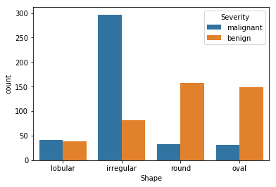
sns.countplot(x='Shape',hue='Severity',data=df)
<matplotlib.axes._subplots.AxesSubplot at 0x7f3ce10ce320>
Inference:
- A large fraction of the
irregular(80%) shaped tumours are malignant. - Most of the
roundandovalshaped tumours are benign. Thus the shape of the tumour is an important feature to be considered.
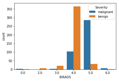
sns.countplot(x='BIRADS',hue='Severity', data=df)
<matplotlib.axes._subplots.AxesSubplot at 0x7f3ce0f72d30>
Inference
- The BIRADS feature is highly skewed with most of the data points concentrated at 4 and 5.
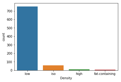
sns.countplot(x='Density', data=df)
<matplotlib.axes._subplots.AxesSubplot at 0x7f3ce10c6240>
Inference:
- Most of the density values in the data set are
low
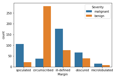
sns.countplot(x='Margin', hue='Severity', data=df)
<matplotlib.axes._subplots.AxesSubplot at 0x7f3ce0d7a208>
Inference:
- Circumscribed masses are likely to be benign
- Spiculated and ill-defined masses are likely to be malignant.
sns.boxplot(x='Severity', y='Age', data=df)
<matplotlib.axes._subplots.AxesSubplot at 0x7f3cde9ccda0>
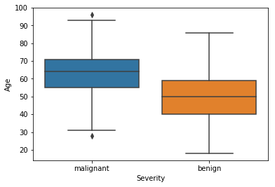
Inference:
- It can be clearly observed that older people are more likely to have a malignant mass
Machine Learning
Handle Categorical Data
Attribute Information
6 Attributes in total (1 goal field, 1 non-predictive, 4 predictive attributes) 1. BI-RADS assessment: 1 to 5 (ordinal, non-predictive!) 2. Age: patient’s age in years (integer) 3. Shape: mass shape: round=1 oval=2 lobular=3 irregular=4 (nominal) 4. Margin: mass margin: circumscribed=1 microlobulated=2 obscured=3 ill-defined=4 spiculated=5 (nominal) 5. Density: mass density high=1 iso=2 low=3 fat-containing=4 (ordinal) 6. Severity: benign=0 or malignant=1 (binominal, goal field!)
As we can see BI-RADS, Density (ordinal) and Shape, Margin(nominal) are all categorical in nature. Thus we need to handle this type of data appropriately.
print(cleanData.head())
   BIRADS   Age  Shape  Margin  Density  Severity
0     5.0  67.0    3.0     5.0      3.0       1.0
1     5.0  58.0    4.0     5.0      3.0       1.0
2     4.0  28.0    1.0     1.0      3.0       0.0
3     5.0  57.0    1.0     5.0      3.0       1.0
4     5.0  76.0    1.0     4.0      3.0       1.0
From the data we can observe that all the categorical features have been transformed into ordinal features. For attributes such as shape and margin which are nominal, ordering does not make sense. Thus we one hot encode these attributes.
Using One Hot Encoding to Handle Categorical data
from sklearn.preprocessing import OneHotEncoder

enc = OneHotEncoder(sparse=False,categories='auto')
shapeFeatureArr = enc.fit_transform(cleanData[['Shape']])
shapeFeatureLabels = ['round', 'oval', 'lobular', 'irregular']
shapeFeature = pd.DataFrame(shapeFeatureArr, columns=shapeFeatureLabels)
shapeFeature

marginFeatureArr = enc.fit_transform(cleanData[['Margin']])
marginFeatureLabels = ['circumscribed', 'microlobulated', 'obscured', 'ill-defined', 'spiculated']
marginFeature = pd.DataFrame(marginFeatureArr, columns=marginFeatureLabels)
marginFeature

dfOHE = pd.concat([cleanData[['BIRADS', 'Age']], shapeFeature, marginFeature, cleanData[['Density','Severity']]],axis=1)
print('Nominal features are one hot encoded and ordinal features are left as is.')
dfOHE.head()
Nominal features are one hot encoded and ordinal features are left as is.
| BIRADS | Age | round | oval | lobular | irregular | circumscribed | microlobulated | obscured | ill-defined | spiculated | Density | Severity | |
|---|---|---|---|---|---|---|---|---|---|---|---|---|---|
| 0 | 5.0 | 67.0 | 0.0 | 0.0 | 1.0 | 0.0 | 0.0 | 0.0 | 0.0 | 0.0 | 1.0 | 3.0 | 1.0 |
| 1 | 5.0 | 58.0 | 0.0 | 0.0 | 0.0 | 1.0 | 0.0 | 0.0 | 0.0 | 0.0 | 1.0 | 3.0 | 1.0 |
| 2 | 4.0 | 28.0 | 1.0 | 0.0 | 0.0 | 0.0 | 1.0 | 0.0 | 0.0 | 0.0 | 0.0 | 3.0 | 0.0 |
| 3 | 5.0 | 57.0 | 1.0 | 0.0 | 0.0 | 0.0 | 0.0 | 0.0 | 0.0 | 0.0 | 1.0 | 3.0 | 1.0 |
| 4 | 5.0 | 76.0 | 1.0 | 0.0 | 0.0 | 0.0 | 0.0 | 0.0 | 0.0 | 1.0 | 0.0 | 3.0 | 1.0 |
From the above table we can observe that the Shape feature has been converted to 4 features namely
round, oval, lobular, irregular and the Margin feature has been converted to 5 features namely
circumscribed, microlobulated, obscured, ill-defined and spiculated.
Further Data processing
Feature Normalisation
We can observe that the range of the Age feature differs from the other categorical features by a large margin. So we normalise our data. After normalising all features are standard normal with mean 0 and unit variance. The features normalisation will be added to sci-kit learn pipeline. It is incorrect to normalise the entire data beforehand as we are using knowledge about the test set to normalise. Therefore information about the test set will leak into the model which is not acceptable.
Removing outliers
No significant outliers can be seen in the data.
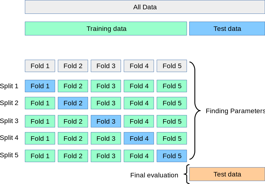
Splitting the Dataset
The dataset needs to be partitioned into training, testing and validation. The training set is used to train the model, the validation set is to optimise model parameters, the testing set is used to evaluate model performance on unseen data. Care needs to be taken so that no bias is introduced in the data.
Since the number of samples are limited (829) k-fold nested cross validation is chosen to be the method to chose an optimal model.
Model Evaluation Metric
Models can be evaluated using a number of metrics like accuracy, precision, recall etc.
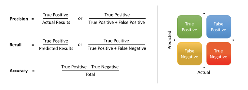
Since we do not want to falsely classify a malignant tumour as benign at any rate, or in other words we want to minimise the number of false negatives we will consider recall as our Model Evaluation Metric.
# Evaluation metric is recall
metric = 'recall'

# Get Inputs and outputs.
X = pd.DataFrame(dfOHE.drop(['Severity'],axis=1))
y = dfOHE['Severity']

from sklearn.model_selection import train_test_split
X_train, X_test, y_train, y_test = train_test_split(X, y, test_size=0.3, random_state=0)
# StandardScaler Object to normalise our inputs.
from sklearn.preprocessing import StandardScaler
scaler = StandardScaler()
Classifiers
We will be considering three classifiers
- Logistic Regression
- Artificial Neural Network
- Support Vector Machine
Logistic Regression
from sklearn.model_selection import cross_validate
from sklearn.model_selection import GridSearchCV
from sklearn.pipeline import make_pipeline
from sklearn.linear_model import LogisticRegression
from sklearn.metrics import *

# First we make a pipeline containing our StandardScaler object and our estimator ie LogisticRegression
clf = make_pipeline(scaler, LogisticRegression(random_state=0,solver='lbfgs'))

# Logistic Regression uses a regularisation hyperparameter 'C'. We find the optimal parameter
# using Cross Validation.
cparams = [ 10**i for i in range(-4,5) ]
params = [{'logisticregression__C': cparams}]
gridLR = GridSearchCV(clf, params, scoring=metric, cv=3)
gridLR.fit(X_train, y_train)
print('Best parameters and Best Score')
print(gridLR.best_params_, gridLR.best_score_)

print('\n\nClassification Report:')
print(classification_report(y_test, gridLR.predict(X_test)))
Best parameters and Best Score
{'logisticregression__C': 0.01} 0.871079476709014


Classification Report:
              precision    recall  f1-score   support

         0.0       0.82      0.76      0.79       134
         1.0       0.74      0.81      0.78       115

   micro avg       0.78      0.78      0.78       249
   macro avg       0.78      0.78      0.78       249
weighted avg       0.79      0.78      0.78       249
Neural Network
from sklearn.neural_network import MLPClassifier
# Parameters to use to find optimal parameters using cross validation
params = {
    'mlpclassifier__hidden_layer_sizes': [(i,j) for i in range(1,10) for j in range(1,10)],
    'mlpclassifier__alpha': [i**10 for i in range(-4,3)]
}
clf = make_pipeline(scaler, MLPClassifier(solver='lbfgs',random_state=0))
gridNN = GridSearchCV(clf, parameter_space,scoring=metric,cv=3, iid=True)

gridNN.fit(X_train, y_train)
print('Best parameters and Best Score')
print(gridNN.best_params_, gridNN.best_score_)

print(classification_report(y_test, gridNN.predict(X_test)))
Best parameters and Best Score
{'mlpclassifier__alpha': 0, 'mlpclassifier__hidden_layer_sizes': (3, 2)} 0.8885015880217785
              precision    recall  f1-score   support

         0.0       0.80      0.80      0.80       134
         1.0       0.77      0.77      0.77       115

   micro avg       0.79      0.79      0.79       249
   macro avg       0.79      0.79      0.79       249
weighted avg       0.79      0.79      0.79       249
Support Vector Machine
from sklearn.svm import SVC

clf = make_pipeline(scaler, SVC())
params = [{'svc__C':[10**i for i in range(-4,4)], 'svc__kernel':['linear', 'poly', 'rbf']}]

gridSVM = GridSearchCV(clf, params, scoring=metric,cv=3, iid=True)
gridSVM.fit(X_train, y_train)
print('Best parameters and best score')
print(gridSVM.best_params_, gridSVM.best_score_)

print(classification_report(y_test, gridSVM.predict(X_test)))
Best parameters and best score
{'svc__C': 0.001, 'svc__kernel': 'linear'} 0.8885012099213553
              precision    recall  f1-score   support

         0.0       0.84      0.73      0.78       134
         1.0       0.73      0.83      0.78       115

   micro avg       0.78      0.78      0.78       249
   macro avg       0.78      0.78      0.78       249
weighted avg       0.79      0.78      0.78       249
We will choose the artificial neural network as our model because it has higher recall than the other models. It can also scale well with more data. ANNs are highly flexible and are a state of the art technique in Machine Learning
Evaluation of the Model
We can see that our model has a false positive rate of just 23% which is much better than the false positive rate of physicians which is at 70%. Thus this model can effectively aid physicians in their diagnosis.
tn, fp, fn, tp = confusion_matrix(y_test, gridNN.predict(X_test)).ravel()

print('False positive rate: %0.2f%%' % (fp*100 / (tp + fp)))
False positive rate: 23.28%
Deploying the model
We now train our model on the entire dataset.
We then serialise it using the pickle library in Python and write it to a file.
This file will be used by a server which is running the model.
# Training the model on the entire data.
gridNN.fit(X,y)
GridSearchCV(cv=3, error_score='raise-deprecating',
       estimator=Pipeline(memory=None,
     steps=[('standardscaler', StandardScaler(copy=True, with_mean=True, with_std=True)), ('mlpclassifier', MLPClassifier(activation='relu', alpha=0.0001, batch_size='auto', beta_1=0.9,
       beta_2=0.999, early_stopping=False, epsilon=1e-08,
       hidden_layer_sizes=(100,), learning_rate='constant',
 ...True, solver='lbfgs', tol=0.0001,
       validation_fraction=0.1, verbose=False, warm_start=False))]),
       fit_params=None, iid=True, n_jobs=None,
       param_grid={'mlpclassifier__hidden_layer_sizes': [(1, 1), (1, 2), (1, 3), (1, 4), (1, 5), (1, 6), (1, 7), (1, 8), (1, 9), (2, 1), (2, 2), (2, 3), (2, 4), (2, 5), (2, 6), (2, 7), (2, 8), (2, 9), (3, 1), (3, 2), (3, 3), (3, 4), (3, 5), (3, 6), (3, 7), (3, 8), (3, 9), (4, 1), (4, 2), (4, 3), (4, 4), (4... 5), (9, 6), (9, 7), (9, 8), (9, 9)], 'mlpclassifier__alpha': [1048576, 59049, 1024, 1, 0, 1, 1024]},
       pre_dispatch='2*n_jobs', refit=True, return_train_score='warn',
       scoring='recall', verbose=0)
# Serializing the model to deploy it.
import pickle
pickle.dump(gridNN, open("modelNN.pkl", "wb"))